9. Pages and Visualizations in Detail

In this chapter, we will take you through the steps involved in performing a detailed quality evaluation in MQC. This will give you a good impression of the functional details of MQC. At the same time, it helps you get accustomed to the tool in a more detailed way than in Quick Start Guide where a quick introduction to the basic functionality of MQC is given.

Building on this and taking into account the dashboards for a project conclusions about the development of software projects are described. Based on these conclusions MQC shows possible reasons for bad quality and helps you deducing actions to carry out for improving quality.

9.1. The MQC dashboard

MQC consists of a default dashboard of overview pages that contain all the important information of your project. The dashboard consists of data and quality pages, showing trend and status respectively, i.e. Quality Trend and Quality Status, as well as Data Trend and Data Status.

The Quality Trend page will give an overview of the quality of your project, whereas the Quality Status, Quality Sunburst and Quality Heatmap page provides an in-depth analysis of Artifacts, i.e. an overview of the quality of each Artifact.

The Quality Model page gives information about the definition of your Quality Properties. It will show you any kind of validation errors.

The Data Status page will give you an overview of the data of your project. By means of Data Details functionality (Data Details) you will get from quality pages, such as Quality Status or Quality Sunburst to the data pages to track the source of a measurement, i.e. going one level down on data source level to Data Trend where you can see your raw data’s trend and get an overview of your related base measures.

The general concept of these pages is that all the visualizations are interactive: If you click into any of the visualizations, the other visualizations will react in a top-down / left-right manner and then show information related to what you have marked. You can do the major selections on the left and top sections of the visualization window and the effect can be seen in the bottom right visualizations.

Marking is cumulative. The marked elements of the first chart will not reset if you mark something in the next chart later. The effect is a combination of marking done in both the charts. To go back to normal state click on the chart where there are no elements.

In dependence of the Project Structures you have imported, the right side panel will display options for filtering the data.

In the following subsections the four main pages as mentioned above are described:

9.2. Data pages

9.2.1. Data Trend

By means of the Data Trend page, you can track the source of a measurement, going one level down compared to the Data Status page, i.e. on data source level. You can see your raw data’s progression and processing getting an overview of your derived and related base measures.

It consists of the following selecting windows:

• Projects (on the top left): Select your project as defined in your project structure. Notice, that you see an availability trend inside the tile. A gradient availability coloring is used that depends on the availability of all measure values for all artifacts shown for the most recent revision.

• Artifacts (Bottom left): Select the artifacts of your choice. By default, all are selected. A gradient availability coloring is used that depends on the availability of the measure values for a single artifact for the most recent revision.

• Measures (next to Artifacts): The count of the measures is with respect to all artifacts and for the last revision. It uses a gradient availability coloring.

• Availability Distribution: This is a bar chart, which bins the amount of available, missing and propagated data for each revision… A categorical availability coloring is used.

The Measure Trend visualization shows per Artifact for each measure value (base measures and derived measures) a trend over all revisions. If a certain revision is selected, the data value for this specific revision is shown only. It is possible to only show the trends for a single or for selected artifacts as well as for selected measures. The Measure Trend visualization uses a dedicated color per trend line for each measure value.

9.2.2. Data Status

The Data Status page offers the following selecting windows:

• Projects (on the top left): Select your project as defined in your project structure. Notice, that you see an availability trend inside the tile. A gradient availability coloring is used that depends on the availability of all measure values for all artifacts shown for the most recent revision.

• Artifacts (Bottom left): Select the artifacts of your choice. By default, all are selected. A gradient availability coloring is used that depends on the availability of the measure values for a single artifact for the most recent revision.

• Availability Distribution: This is a bar chart, which bins the amount of available, propagated, missing data and data to which a default value is applied for each revision. It uses a categorical availability coloring.

The Availability Treemap is the reacting window to the selections (intersections) made by the marking in the selecting windows mentioned above. It also uses a categorical availability coloring.

9.3. Quality pages

9.3.1. Quality Status

The Quality Status page provides an in-depth analysis of Artifacts. Therefore, it will give an overview of the quality of each Artifact.

Selecting windows are:

• Projects (on the top left): Select your project as defined in your project structure for which you want to see quality. If you have defined only a single project, it is selected by default. You can reset the marking for the entire page at any point by clicking on this tile. Notice, that you see a quality trend over all revisions inside the tile. A gradient quality coloring is used that depends on the overall quality for all artifacts, shown for the most recent revision.

• Artifacts (Bottom left): Select the Artifacts of your choice. By default, all are selected. The values within the tiles are always related to the latest revision. A gradient quality coloring is used that depends on the quality for each artifact, shown for the most recent revision.

• Quality properties (next to Artifacts): Select the Quality Property. Note, that the Properties tiles are listed in ascending order of quality measure. If the quality measure cannot be computed, then it appears in the bottom of the list with an empty value. The values within the tiles are always of the latest revision. A gradient quality coloring is used.

• Quality Bin Distribution (top): The computed quality property measures are mainly binned as Good, Acceptable and Bad. By marking the bins in this visualization you can do selections based on the computed quality status of all quality properties per revision. You can also select the revision of the data by selecting all the bins of the same revision. For example, if you select the green bin of the latest revision on the Quality Bin Distribution visualization, the reacting window shows an overview of all information related to good quality measures for this revision. For the bins a categorical quality coloring is used.

The reacting window is a heatmap visualization plotted for each Artifact against each Quality Property. Each Quality Property tile has a gradient quality coloring, which represents the quality value for the particular property. Based on the marking from the selecting windows, the boxes in the heatmap are highlighted.

You can now start identifying the reason for bad quality. The general concept of identifying issues is to click on (or hover over) red quality bins or tiles. When clicking on red, data that corresponds to green and yellow bins is excluded from the chart visualizations to receive a first impression of the reason for bad quality, concretely the quality properties that have failed.

9.3.2. Quality Sunburst

The Quality Sunburst page will give an overview of the quality of your project.

The selecting windows are the same as on the Quality Status page, just the main visualization shows the sunburst visualization where the outer ring consists of all quality properties defined by the quality model (see section Quality Properties).

9.3.3. Quality Heatmap

The Quality Heatmap page will give an overview of the quality of your project.

The selecting windows are the same as on the Quality Status page, just the main visualization shows a more detailed heat map visualization, where quality properties and artifacts are visualized with their aggregation and respective “size” (weight).

9.3.4. Quality Trend

The Quality Trend page will give an overview of the quality of your project.

The selecting windows are the same as on the Quality Status and Quality Sunburst page.

Quality Trend by Artifact and Quality Trend by Property are the reacting windows. These line chart visualizations are updated based on your previous selections.

The trend visualizations use a categorical coloring, so each line representing an Artifact resp. a quality property uses a dedicated color.

9.4. Tool pages

9.4.1. MXAM Tool Page

Besides the standard data and quality pages, MQC provides an additional tool page showing details on data provided by MXAM.

From the menu bar choose Tools/MQC Tool Pages/Add MXAM Details Page to add the MXAM tool page.

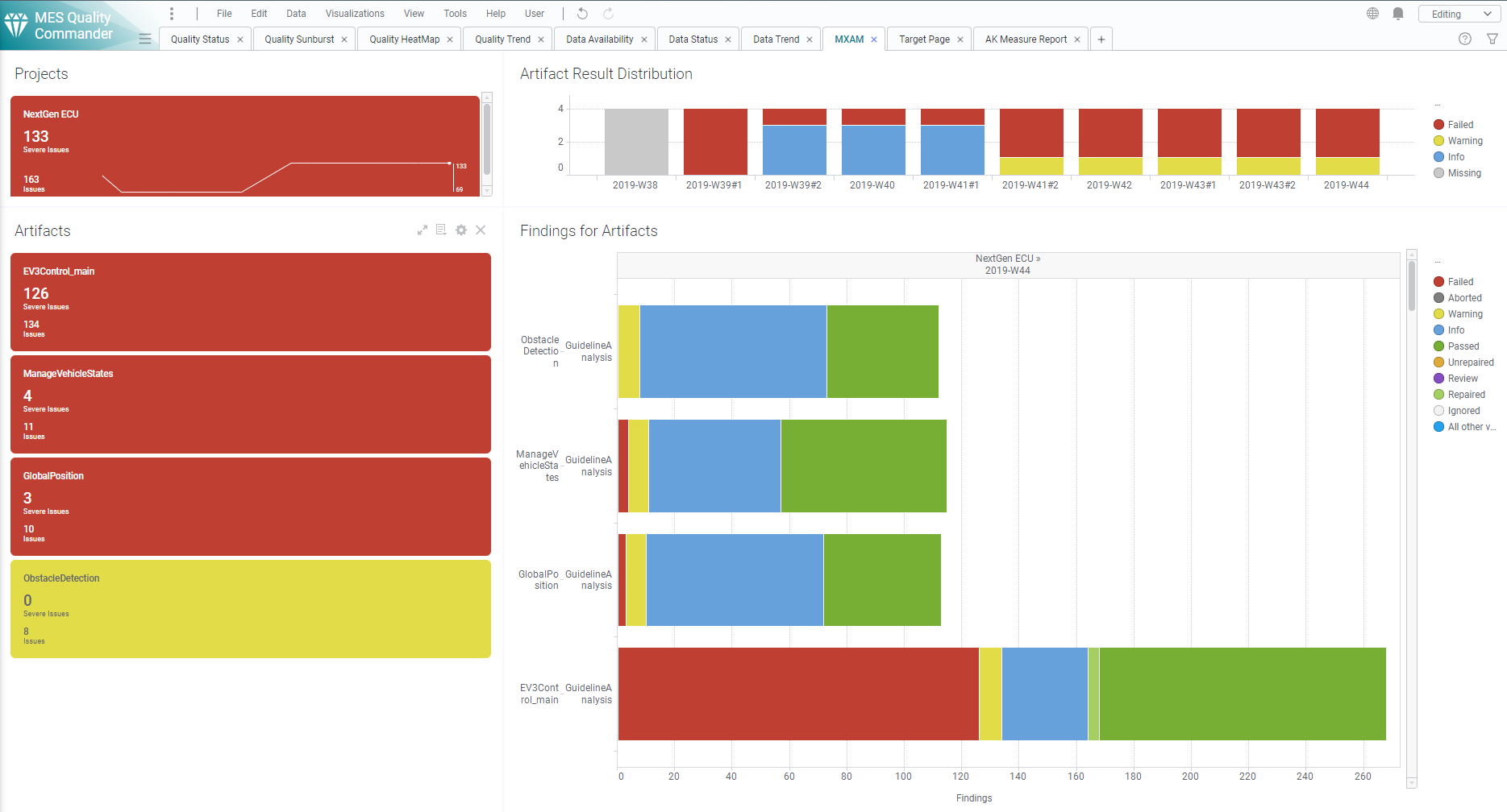
Figure 9.1 MXAM Details Page showing Findings per Artifact and Revision

The main visualization (horizontal bar chart) shows for each artifact all findings based on FindingCount (e.g. Failed, Passed, Warning etc. as provided by the MXAM report). As long as data for multiple revisions is imported and no particular revision is marked respectively, the visualization offers to scroll between revisions to get the finding status for a certain point in time.

The Artifact KPI on the left-hand side shows a tile for each artifact colored according to the worst finding result for this artifact (using the MXAM results order), i.e. in Figure 9.1 all artifacts have failed checks, but no findings for Canceled, Aborted or Review. So, all tiles are colored red.

The MXAM result coloring is shown in the following figure:

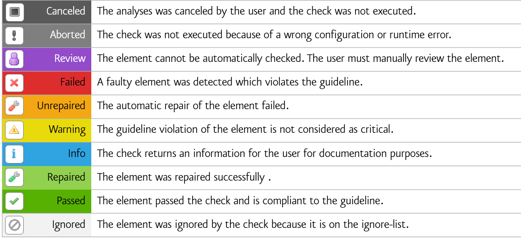
Figure 9.2 List of all existing MXAM results

Additionally each tile shows per artifact:

• the number of severe issues (sum of Aborted, Canceled, Failed, Review and Unrepaired findings)

• the number of issues (servere issues plus Warning)

The Project KPI chart on the top-left of the page shows the color of the worst finding over all artifacts as well as the number of severe issues and issues summed up over all artifacts.

The distribution chart (top-right) shows for each revision the number of artifacts binned according to their worst findings. For the example in Figure 9.1 this means there are four artifacts in total, all of them with Failed findings.

By these means the user gets an overview on

• how many findings per artifact exist

• which findings per artifact exist

• what are the worst findings to concentrate on first (for each artifact and for the whole project)

• and how this has evolved over time (e.g. from project start time until actual date).

9.4.2. MXRAY Tool Page

Besides the standard data and quality pages, MQC provides an additional tool page showing details on data provided by MXRAY.

From the menu bar choose Tools/MQC Tool Pages/Add MXRAY Details Page to add the MXRAY tool page.

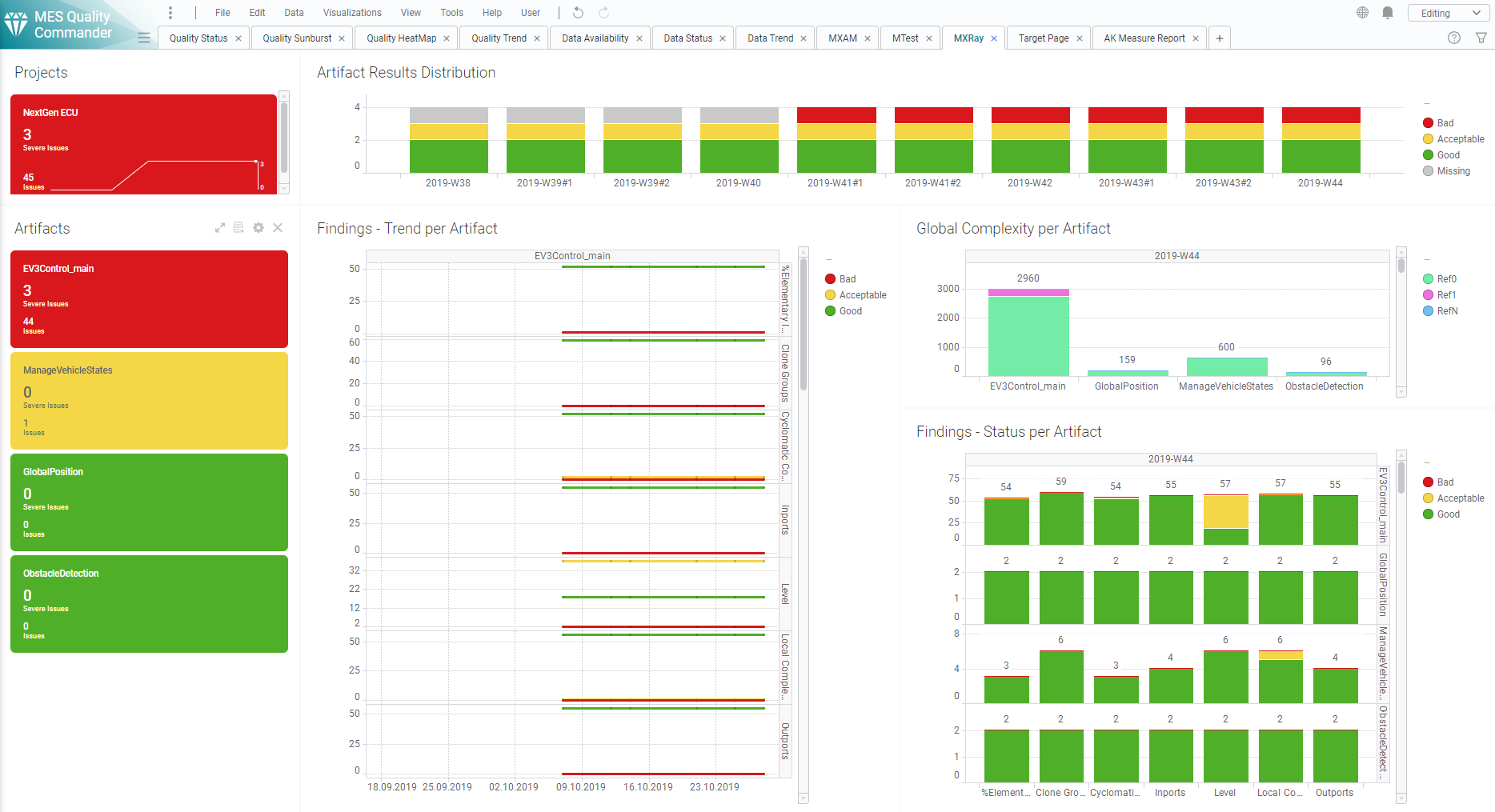
Figure 9.3 MXRAY Details Page showing Findings in Trend and Status and Global Complexity per Artifact and Revision

This page contains three main visualizations:

• Global Complexity per Artifact

• Status of subsystem results per base measure and Artifact

• Trend of subsystem results per base measure and Artifact

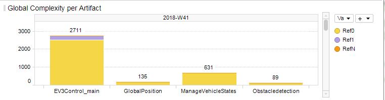
Figure 9.4 MXRAY Global Complexity per Artifact

The Global Complexity visualization (Figure 9.4) shows for each artifact the stacked values of Ref0, Ref1 and RefN, where:

• Ref0 is the global complexity of the model itself excluding all referenced libraries resp. models

• Ref1 includes the global complexity of referenced libraries/models exactly one time (each library/model is counted once)

• RefN includes the global complexity of referenced libraries/models whereas a complexity value is added for each occurence (each library/model may count multiple times depending on how often a library/model is referenced)

The global complexity visualization shows the values for Ref1 and RefN just in addition to Ref0, which means

• Ref1 (as shown) = Ref1 (as measured) - Ref0

• RefN (as shown) = RefN (as measured) - Ref1

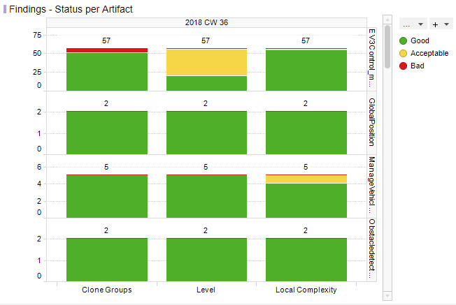
Figure 9.5 MXRAY Subsystems Results Status per Base Measure per Artifact

Figure 9.5 shows reported results per base measure per artifact. The user gets an overview on how many subsystems per artifact are stated good, acceptable or bad for all metrics provided by the imported report:

• Local Complexity

• Level

• CloneGroups (Good and Bad only, see adaptation of clone group values as previously described)

Note

As long as data for multiple revisions is imported and no particular revision is marked respectively, all status visualizations (bar charts) offer the option to scroll between revisions.

The third main visualization showing the trend of subsystem results (see Figure 9.6) shows the same metrics as listed above, but rather its evolution over time than the status for a certain revision.

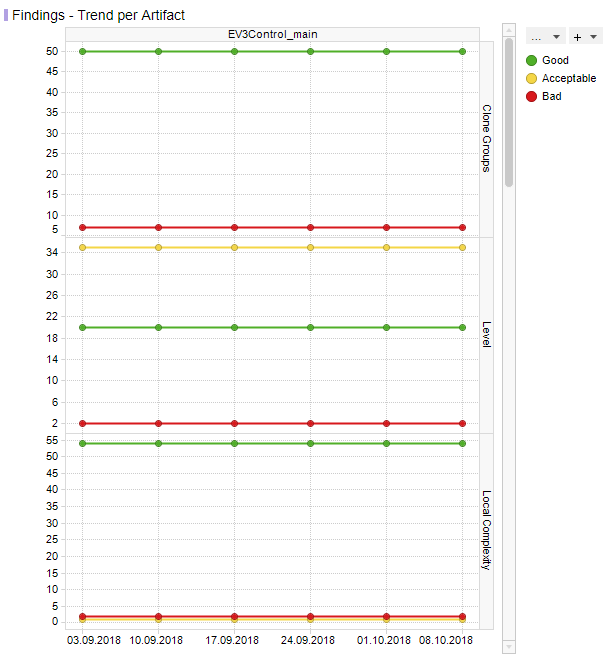
Figure 9.6 MXRAY subsystem results Trend per Base Measure per Artifact

With that the user is able to see the number of good subsystems that increase during the project runtime while the number of acceptable and bad subsystems decreases. It is also possible to detect an increase of the overall number of subsystems per model at a certain point in time (e.g. if a model was extended during development).

If there are multiple selected artifacts (or no specific one), the user is able to scroll between artifacts to see the trend figures for a particular artifact.

The Artifact KPI on the left-hand side shows a tile for each artifact colored according to the number of found severe issues or issues, respectively.

• Severe Issues:

  Sum of all Bad measures per artifact.

• Issues:

  Sum of all Bad AND Acceptable measures per artifact.

If there is any Severe Issue, which means a base measure (e.g. Level or Local Complexity) with a variable value of Bad > 0, the artifact tile is colored red.

If there are no Severe Issues, but Issues (which means a base measure with a variable value of Acceptable > 0) are found, the artifact tile is colored yellow.

All other artifact KPIs are colored green.

The Project KPI chart on the top-left of the page shows the color of the worst result over all artifacts as well as the overall number of Severe Issues and Issues for the whole project.

The distribution chart (top-right) shows for each revision the number of artifacts binned according to their worst result.

By these means the user gets an overview on

• the global complexity of each artifact compared to all other artifacts

• how many issues (e.g. subsystems with problems) per artifact exist

• which issues per artifact exist (e.g. subsystems with bad local complexity)

• what are the worst issues to concentrate on first (for each artifact and for the whole project)

• and how this has evolved over time (e.g. from project start time until actual date).

9.4.3. MTest Tool Page

To dig more into details from the Base Measures and Quality properties of the MTest tool, MQC provides an additional MTest Details page.

From the menu bar choose Tools/MQC Tool Pages/Add MTest Details Page to add the MTest tool page.

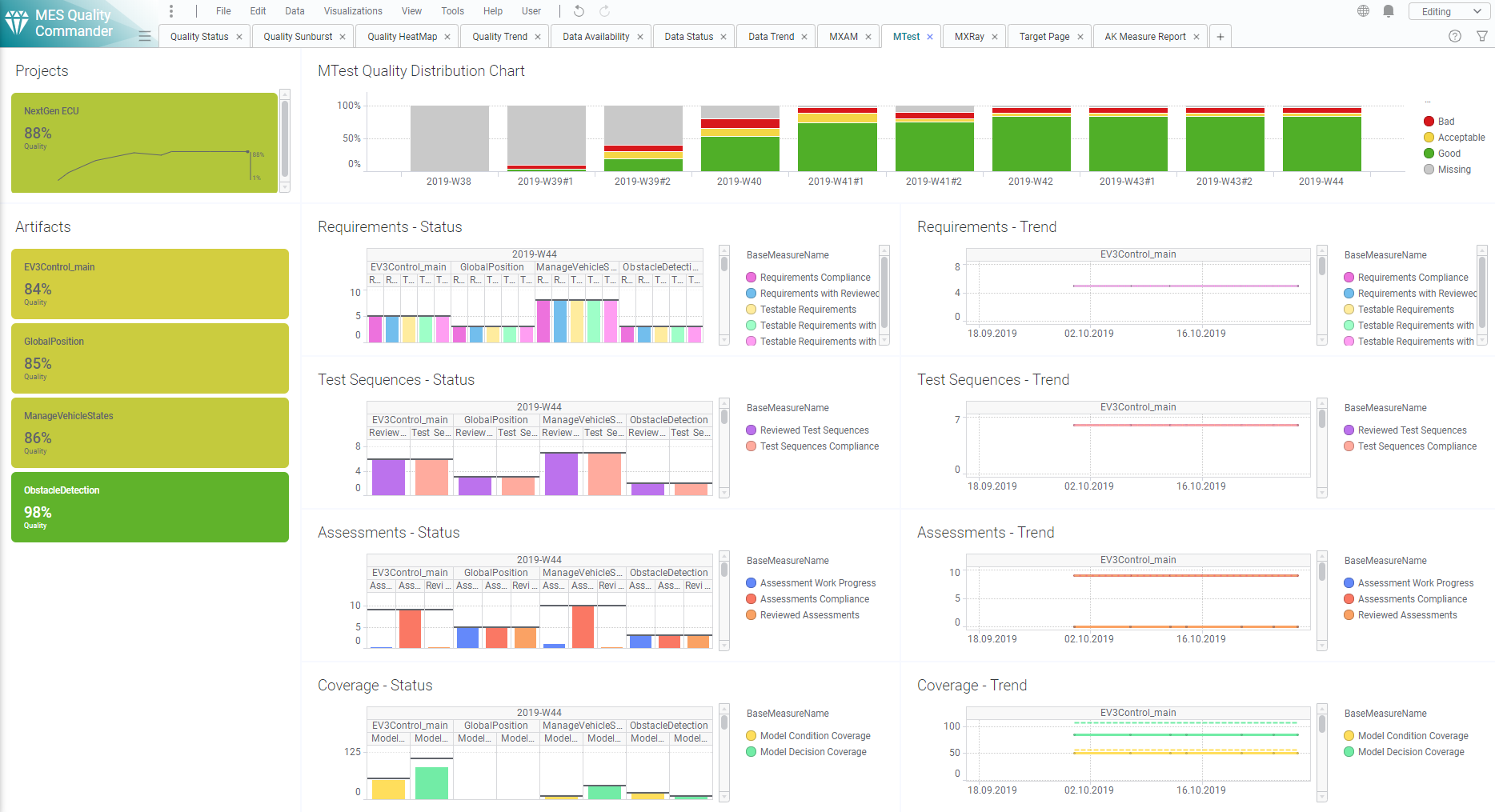
Figure 9.7 MTest Details Page showing Trend and Status

The visualized data is structured by

• Requirements

• Test Sequences

• Assessments and

• (Structural) Coverage.

For each Base Measure MTest provides two values, read and visualized by MQC:

• Total, e.g. the total number of reviewed Test Sequences, and

• Reached, e.g. the actual number of reviewed Test Sequences

Both values are shown in Status (see Figure 9.8) as well as in Trend (see Figure 9.9).

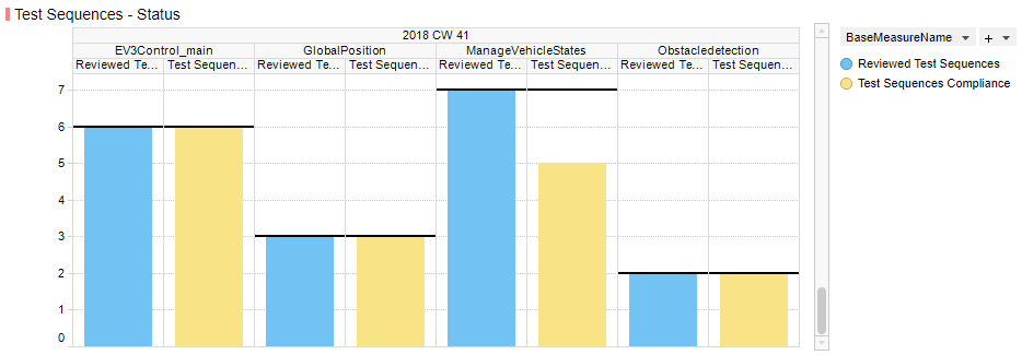
Figure 9.8 Measure Status visualization for Test Sequences

Each status diagram shows the Reached values of the imported base measures as bar charts per artifact. The Total values are shown as horizontal line (i.e. like a target to be reached) for each measure bar.

As long as data for multiple revisions is imported and no particular revision is selected respectively, MQC offers to scroll between revisions. The Artifact KPI selector (on the left-hand side) is used to limit the shown data for particular artifacts.

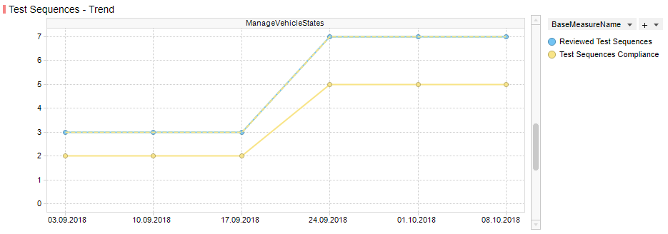
Figure 9.9 Measure Trend visualization for Test Sequences

Each trend diagram shows the Reached values of the imported base measures as a trend line over revisions per artifact. The Total values are shown as an additional dotted line (i.e. like a target to be reached) for each shown measure trend.

If multiple artifacts (or no specific artifact) are (is) selected, the user is able to scroll between artifacts to see the trend figures for a particular artifact.

Artifact KPI selector (left-hand side), Project KPI selector (top-left) and Bin Distribution chart (top-right) are showing quality as on the MQC quality pages.

By these means the user gets an overview on

• the progress of the functional tests

• the current status of the functional tests

• certain Artifact(s)

• a certain test area.

9.4.4. Polyspace Tool Page

MQC provides an additional tool page showing details on data provided by Polyspace.

From the menu bar choose Tools/MQC Tool Pages/Add Polyspace Details Page to add the Polyspace tool page.

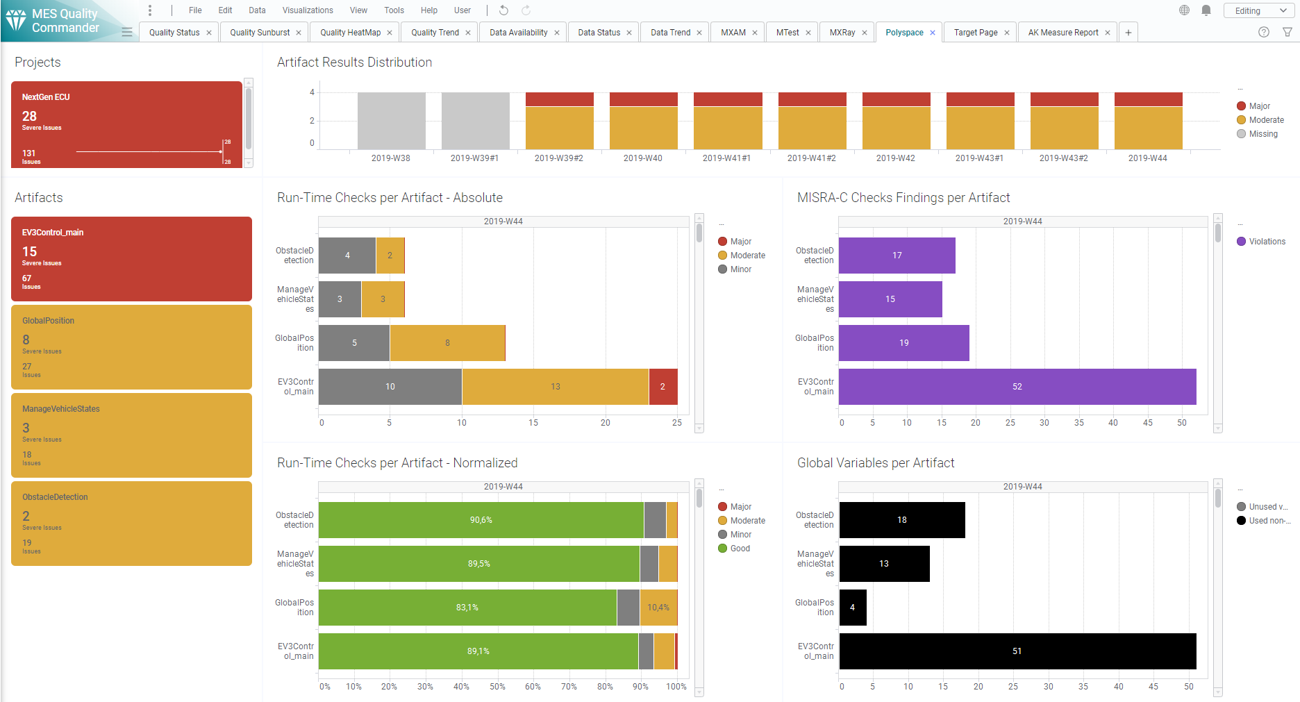
Figure 9.10 Polyspace Details Page

This page contains four main visualizations:

• Run-Time Checks per Artifact - Absolute

• Run-Time Checks per Artifact - Normalized

• MISRA-C Checks Findings per Artifact

• Global Variables per Artifact

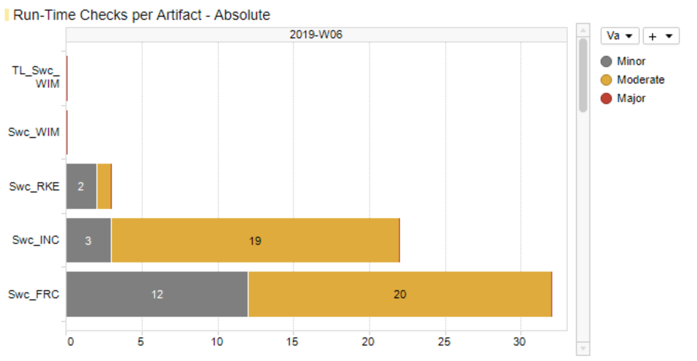
Figure 9.11 Polyspace Run-Time Checks per Artifact - Absolute

The first Run-Time Checks visualization (Figure 9.11) - top-left of the main visualization area - shows for each artifact the stacked absolute values of all findings excluding the number of green checks:

• Run-Time Checks.Major (Number of Red Checks)

• Run-Time Checks.Moderate (Number of Orange Checks)

• Run-Time Checks.Minor (Number of Gray Checks)

This directly indicates the amount of still open and to be solved issues per artifact without being concealed by a huge number of Run-Time Checks.Good.

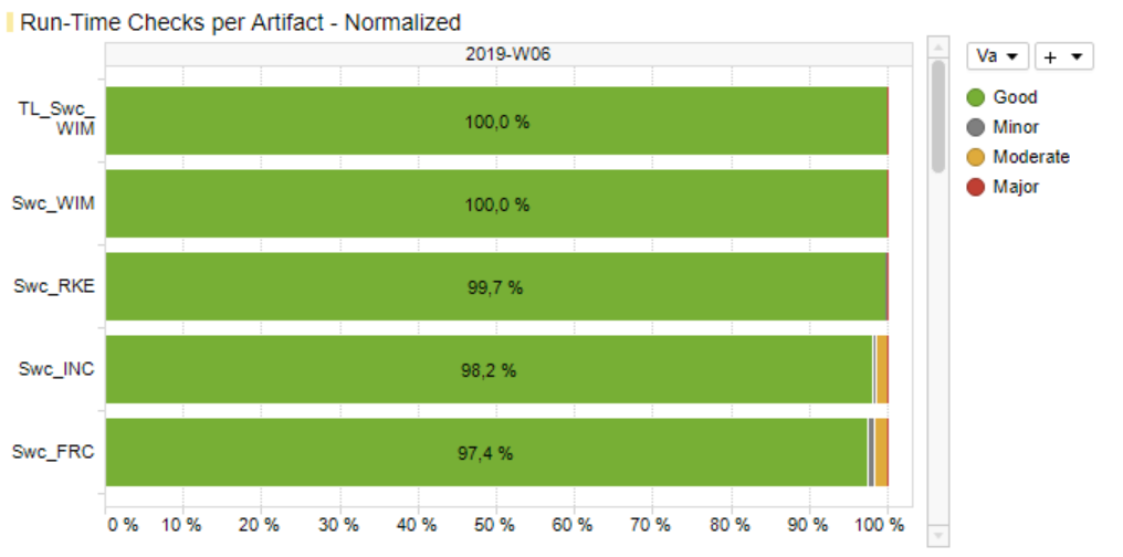
Figure 9.12 Polyspace Run-Time Checks per Artifact - Normalized

Figure 9.12 - at the bottom-left - also shows Run-Time Checks, but this time the relative share (in percent) of each result including the number of green checks compared to the overall number of findings per artifact.

The third main visualization (Figure 9.13) - top-right - shows the absolute number of coding rule violations per artifact.

If a Polyspace report contains different types of coding rule checks, e.g. additionally custom rules, all violations found per artifact will be already summed up by the Polyspace adapter to MISRA-C Checker.Violations and will be shown as one value on the MQC data pages as well as on the Polyspace tool page.

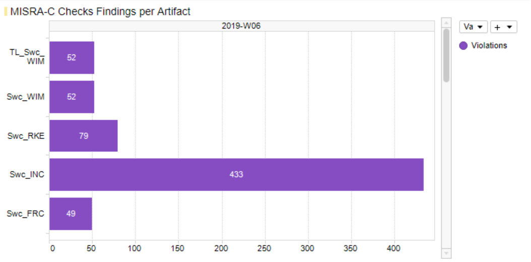
Figure 9.13 Polyspace Coding Rule Violations per Artifact

The forth main visualization (Figure 9.14) - bottom-right - shows for each artifact the stacked absolute numbers of global variables:

• Unused variable (grey)

• Used non-shared variable (black)

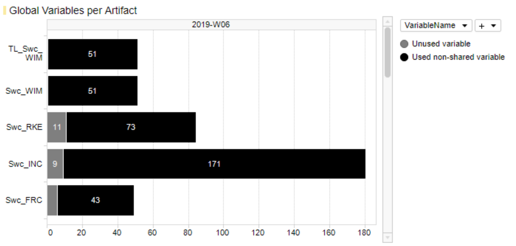
Figure 9.14 Polyspace Global Variables per Artifact

As long as data for multiple revisions is imported and no particular revision is marked respectively selected, all main visualizations offer to scroll between revisions to get the Polyspace results for a certain point in time.

The Artifact KPI on the left-hand side shows a tile for each artifact colored according to the number of found issues or severe issues, respectively.

• Severe Issues:

  Sum of all Run-Time Checks.Major and Run-Time Checks.Moderate findings per artifact.

• Issues:

  Sum of all Run-Time Checks.Major, Run-Time Checks.Moderate and MISRA-C Checker.Violations findings per artifact.

If there is any Major finding, the artifact tile is colored red.

If there is no Major but Moderate finding, the artifact tile is colored orange.

If there are no Severe Issues at all, but Issues (which means Violations > 0), the artifact tile is colored violet.

All other artifact KPIs are colored green.

The Artifact KPI on the left-hand side shows a tile for each artifact colored according to the number of found Severe Issues and Issues respectively. For the example in Figure 9.3 this means that within the current (last) revision there are four artifacts in total, one of them with severe issues (red bin), one with issues only (yellow bin) and two artifacts with no issues at all (green bins).

The Project KPI chart on the top-left of the page shows the color of the worst result over all artifacts as well as the overall number of Severe Issues and Issues for the whole project.

The distribution chart (top-right) shows for each revision the number of artifacts binned according to their worst result.

9.5. Color Schemes

On Quality Pages (i.e. Quality Status page, Quality Sunburst page and Quality Trend page), MQC uses the traffic light color scheme:

	Good	All quality properties with an evaluated quality between 80% - 100%
	Acceptable	All quality properties with an evaluated quality between 20% - 80%
	Bad	All quality properties with an evaluated quality between 0% - 20%
	Missing	Quality cannot be evaluated because of missing quality measure values

Gradient	Description
Coloring
	100% quality	A gradient coloring is mainly used for certain elements that have a computed or aggregated quality value assigned (e.g. for projects, artifacts and quality properties)
	50% quality
	0% quality
	No quality value available

On Availability Pages (i.e. Data Status page and Data Trend page) the MQC uses a blue coloring scheme. This means you can easily distinguish between available data in blue and missing data in grey.

Categorical	Description
Coloring
Available	Measure data is available for a certain revision
Default	Measure value was missing, hence filled up with a previously defined default value
Propagated	Measure was missing, but could be propagated from previous revision
Missing	Measure data is missing for a certain revision

Gradient	Description
Coloring
	100% data available	A gradient coloring is mainly used for certain elements that have an aggregated availability value assigned (e.g. projects and artifacts)
	0% data available

9.6. Marking

The purpose of marking is to restrict the shown data to the interesting parts.

The following should be considered while using marking:

• When marking one or multiple elements of a visialization, the data that corresponds to other, not marked, elements are excluded from all visualizations.

  

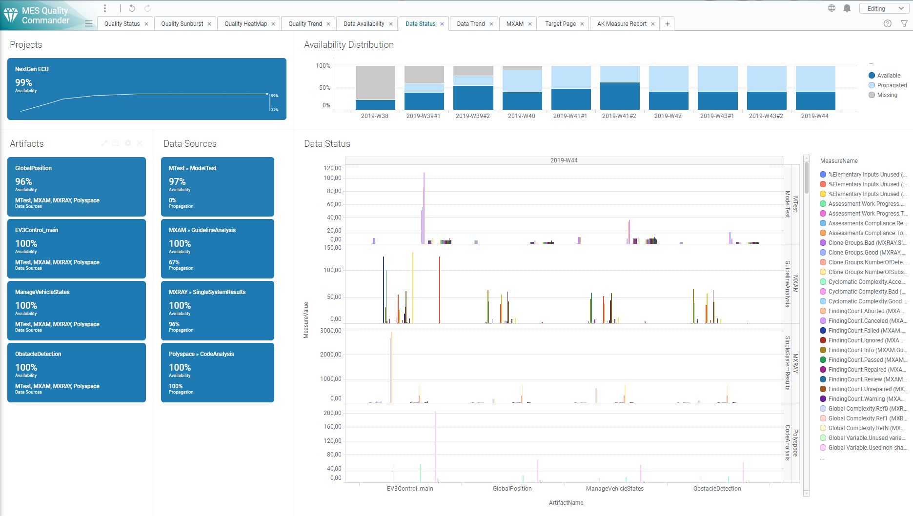
  Figure 9.15 Data Status page without any marking

  

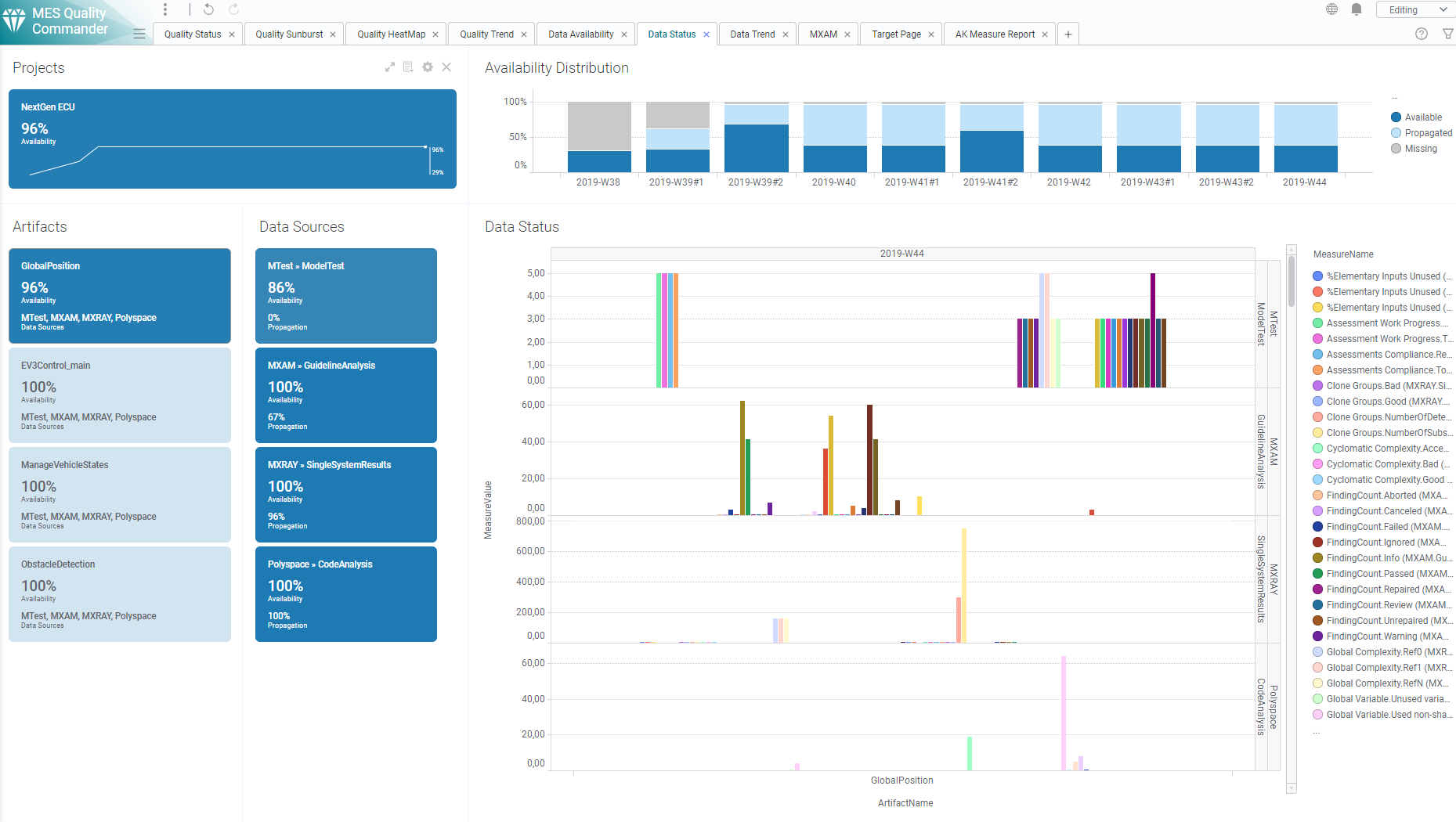
  Figure 9.16 Using artifact marking on Data Status: All other visualizations show only data related to the selected artifact (GlobalPosition)

  As seen in Figure 9.16, by marking data in one visualization except the main visualization, only data representing this marking selection is shown in each of the other visualizations.

• Please note that marking works cumulative. That means further marking without resetting will reduce the resulting set of data even more. To mark multiple elements in the same visualization, press and hold Ctrl before clicking on another element. It is also possible to draw a rectangle enclosing the interesting parts by clicking and holding down the mouse button. (e.g. in Distribution charts).

• Resetting the markings can be achieved by clicking on the Project KPI tile.

• On Status pages (Data Availability, Data Status, Quality Status, Quality Sunburst, Quality Heatmap), a revision is marked with just one click in the distribution visualization. With a second click the quality bin is marked.

• On trend pages (Data Trend, Quality Trend) quality bins can be marked for all revisions with one click.

  

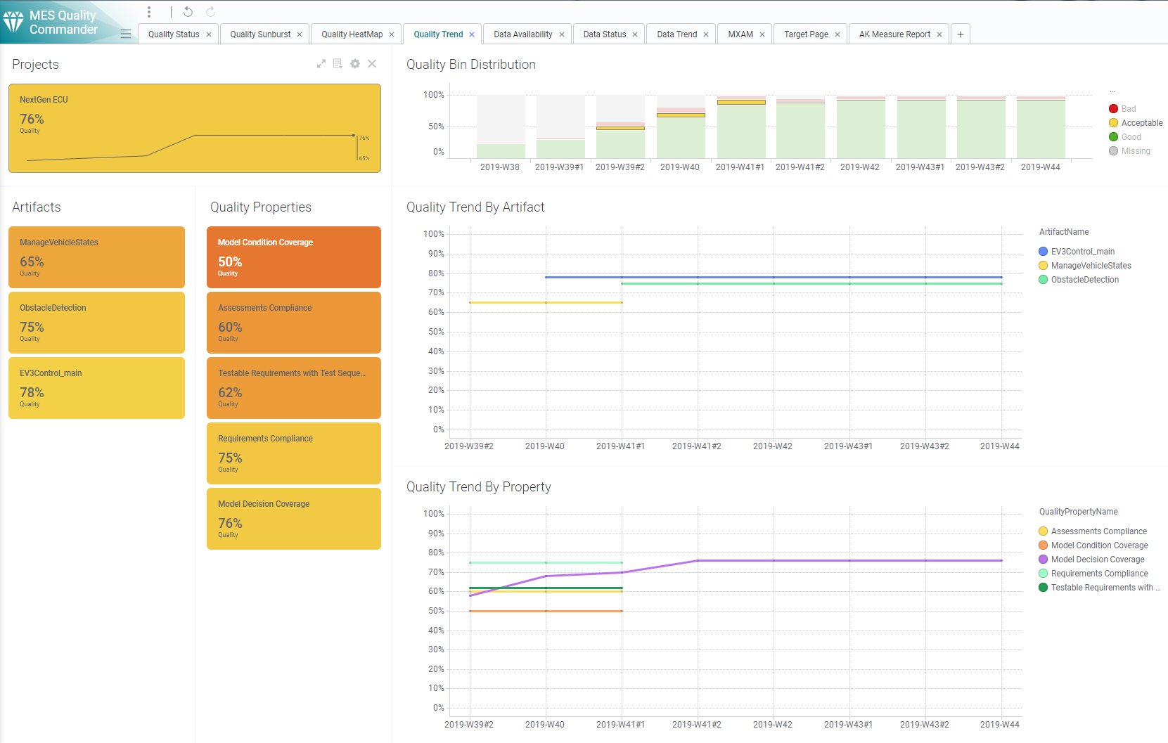
  Figure 9.17 On the Quality Trend page the first click on an quality bin will select the quality bins for all revisions

• Artifact and revision marking on quality or data pages will result in the marking on other quality and data pages.

  

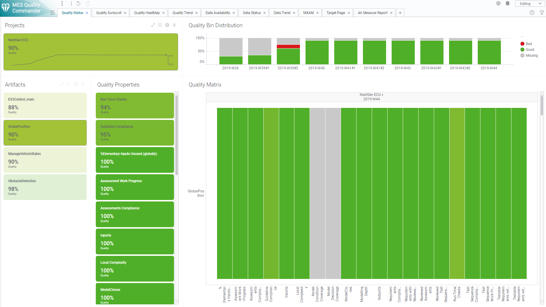
  Figure 9.18 Quality Status page after marking GlobalPosition on data pages (see Figure 9.16)